Tips and Tricks for the Project

In this lesson, you've acquired some new tools to help you find and track the lane lines. By all means, you are welcome and encouraged to use the techniques you used in the very first project. Here are some tips for the upcoming project.

Camera Calibration

The calibration images in the lesson exercise were taken with a different camera setting and a different chessboard pattern than the calibration images for the project. You need to set your chessboard size to 9x6 for the project instead of 8x6 as in the lesson.

Do your curvature values make sense?

We're not expecting anything like perfection for this project, but a good check on whether or not your perspective transform worked as expected, your conversion from pixel space to world space was correct, and that you successfully calculated the radius of curvature is whether or not your results are roughly consistent with reality.

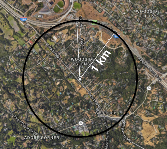
Here is an image from Google maps of where the project video was made (just northwest of the Udacity office!). Here, I've drawn a circle to coincide with the first left curve in the project video. This is a very rough estimate, but as you can see, the radius of that circle is approximately 1 km. You don't need to tune your algorithm to report exactly a radius of 1 km in the project, but if you're reporting 10 km or 0.1 km, you know there might be something wrong with your calculations!

Here are some other tips and tricks for building a robust pipeline:

Offset

You can assume the camera is mounted at the center of the car, such that the lane center is the midpoint at the bottom of the image between the two lines you've detected. The offset of the lane center from the center of the image (converted from pixels to meters) is your distance from the center of the lane.

Tracking

After you've tuned your pipeline on test images, you'll run on a video stream, just like in the first project. In this case, however, you're going to keep track of things like where your last several detections of the lane lines were and what the curvature was, so you can properly treat new detections. To do this, it's useful to define a Line() class to keep track of all the interesting parameters you measure from frame to frame. Here's an example:

# Define a class to receive the characteristics of each line detection
class Line():
    def __init__(self):
        # was the line detected in the last iteration?
        self.detected = False  
        # x values of the last n fits of the line
        self.recent_xfitted = [] 
        #average x values of the fitted line over the last n iterations
        self.bestx = None     
        #polynomial coefficients averaged over the last n iterations
        self.best_fit = None  
        #polynomial coefficients for the most recent fit
        self.current_fit = [np.array([False])]  
        #radius of curvature of the line in some units
        self.radius_of_curvature = None 
        #distance in meters of vehicle center from the line
        self.line_base_pos = None 
        #difference in fit coefficients between last and new fits
        self.diffs = np.array([0,0,0], dtype='float') 
        #x values for detected line pixels
        self.allx = None  
        #y values for detected line pixels
        self.ally = None  

You can create an instance of the Line() class for the left and right lane lines to keep track of recent detections and to perform sanity checks.

Sanity Check

Ok, so your algorithm found some lines. Before moving on, you should check that the detection makes sense. To confirm that your detected lane lines are real, you might consider:

• Checking that they have similar curvature
• Checking that they are separated by approximately the right distance horizontally
• Checking that they are roughly parallel

Look-Ahead Filter

Once you've found the lane lines in one frame of video, and you are reasonably confident they are actually the lines you are looking for, you don't need to search blindly in the next frame. You can simply search within a window around the previous detection.

For example, if you fit a polynomial, then for each y position, you have an x position that represents the lane center from the last frame. Search for the new line within +/- some margin around the old line center.

If you need a reminder on how this works, make sure to go back and check the Finding the Lines: Search from Prior quiz from last lesson!

Then check that your new line detections makes sense (i.e. expected curvature, separation, and slope).

Reset

If your sanity checks reveal that the lane lines you've detected are problematic for some reason, you can simply assume it was a bad or difficult frame of video, retain the previous positions from the frame prior and step to the next frame to search again. If you lose the lines for several frames in a row, you should probably start searching from scratch using a histogram and sliding window, or another method, to re-establish your measurement.

Smoothing

Even when everything is working, your line detections will jump around from frame to frame a bit and it can be preferable to smooth over the last n frames of video to obtain a cleaner result. Each time you get a new high-confidence measurement, you can append it to the list of recent measurements and then take an average over n past measurements to obtain the lane position you want to draw onto the image.

Drawing

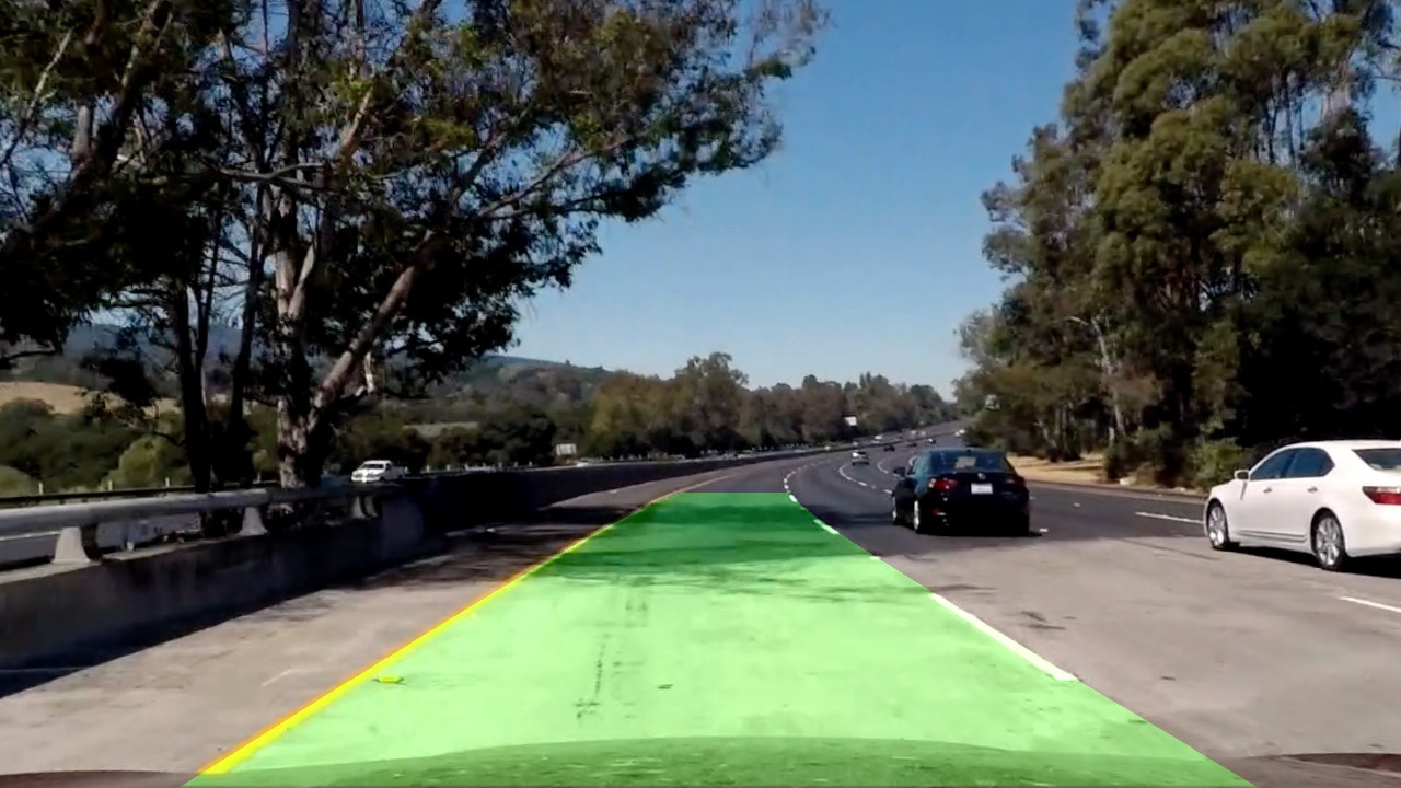
Once you have a good measurement of the line positions in warped space, it's time to project your measurement back down onto the road! Let's suppose, as in the previous example, you have a warped binary image called warped , and you have fit the lines with a polynomial and have arrays called ploty , left_fitx and right_fitx , which represent the x and y pixel values of the lines. You can then project those lines onto the original image as follows:

# Create an image to draw the lines on
warp_zero = np.zeros_like(warped).astype(np.uint8)
color_warp = np.dstack((warp_zero, warp_zero, warp_zero))

# Recast the x and y points into usable format for cv2.fillPoly()
pts_left = np.array([np.transpose(np.vstack([left_fitx, ploty]))])
pts_right = np.array([np.flipud(np.transpose(np.vstack([right_fitx, ploty])))])
pts = np.hstack((pts_left, pts_right))

# Draw the lane onto the warped blank image
cv2.fillPoly(color_warp, np.int_([pts]), (0,255, 0))

# Warp the blank back to original image space using inverse perspective matrix (Minv)
newwarp = cv2.warpPerspective(color_warp, Minv, (image.shape[1], image.shape[0])) 
# Combine the result with the original image
result = cv2.addWeighted(undist, 1, newwarp, 0.3, 0)
plt.imshow(result)